# Preliminaries ####
# remove everything from the environment
rm(list = ls())

# set the working directory:
setwd("~/methods/") # adjust the directory address accordingly8 Regression
In our last lecture, we covered the fundamentals of regression. Today, we will continue to applying regression in R. We will begin by exploring the basics to build a solid foundation.
Let’s revisit the intuitive example we discussed last week: the relationship between Infant Mortality Rate and Female Life Expectancy.
8.1 Preliminaries
# require the packages
library(tidyverse)
── Attaching core tidyverse packages ──────────────────────── tidyverse 2.0.0 ──
✔ dplyr 1.1.4 ✔ readr 2.1.5
✔ forcats 1.0.0 ✔ stringr 1.5.1
✔ ggplot2 3.5.1 ✔ tibble 3.2.1
✔ lubridate 1.9.3 ✔ tidyr 1.3.1
✔ purrr 1.0.2
── Conflicts ────────────────────────────────────────── tidyverse_conflicts() ──
✖ dplyr::filter() masks stats::filter()
✖ dplyr::lag() masks stats::lag()
ℹ Use the conflicted package (<http://conflicted.r-lib.org/>) to force all conflicts to become errorsNext, import the dataset World in 2010.
# Import the dataset: World in 2010 ####
# import the data:
df <- read.csv("data/world_in_2010.csv")
8.2 Female Life Expectancy and Mortality Rate
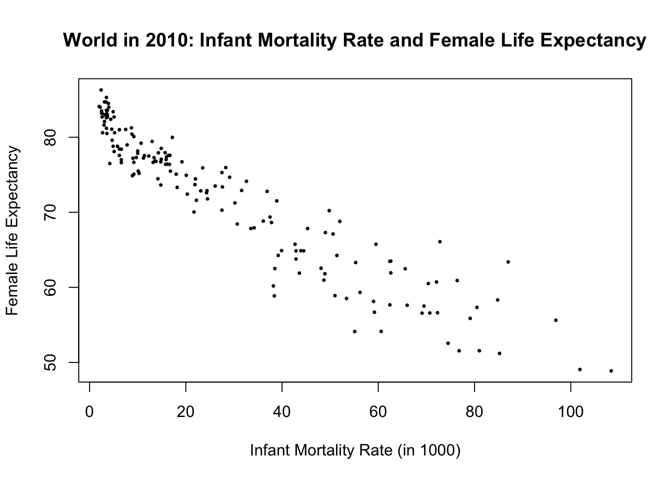
We will explore the relationship between Infant Mortality Rate and Female Life Expectancy. Remember, there is no reason to assume that one variable causes the other. Since there is no clear outcome or explanatory variable, we will simply designate one as the predicted variable and the other as the predictor. As we did last week, let’s place Infant Mortality Rate on the x-axis and Female Life Expectancy on the y-axis.
plot(df$Infant_Mortality_Rate, df$Life_exp_female,
     main = "World in 2010: Infant Mortality Rate and Female Life Expectancy",
     xlab = "Infant Mortality Rate (in 1000)",
     ylab = "Female Life Expectancy",
     pch = 16, # change points from hollow circles to filled circle
     cex = 0.5 # make the points smaller (half in size)
     )
8.3 Regression Equation
Next, we are going to fit a regression line to Figure 8.1. Let’s type our regression equation first:
\[ FemLifeExp = \alpha + \beta * InfMortRate \tag{8.1}\]
For simplicity we could also write it as: \[ Y = \alpha + \beta * X \tag{8.2}\]
where \(Y\) is Life_exp_female and \(X\) is Infant_Mortality_Rate.
Equation 8.2 represents the generic equation we will use for all regression analyses (with some adjustments when required).
When we are telling R to fit the best line, we are asking it to estimate the coefficients of \(\alpha\) and \(\beta\).
For running a regression, we will use the base R function lm(), which stands for linear model. Following the structure in {#eq-form1}, I need to specify my predicted variable, Life_exp_female. R knows that an \(\alpha\) is needed, so we do not need to type anything for it. My predictor variable is Infant_Mortality_Rate. To separate the left and right hand-side of the equation, I use a tilda (~). You can read this formula as “Female Life Expectancy as a function of Infant Mortality Rate”.
# linear model : ####
lm(df$Life_exp_female ~ df$Infant_Mortality_Rate)
Call:
lm(formula = df$Life_exp_female ~ df$Infant_Mortality_Rate)

Coefficients:
             (Intercept)  df$Infant_Mortality_Rate
                 81.9260                   -0.3414
R brought us the coefficients for \(\alpha = 81.9260\) and \(\beta = -0.3414\). Recall that \(\alpha\) is also called the intercept.
More common code: without the $ notation
We can also specify the dataset and just type the variables (without using the $ notation). We will most often type in this way.
# linear model :
lm(Life_exp_female ~ Infant_Mortality_Rate, data = df)
Call:
lm(formula = Life_exp_female ~ Infant_Mortality_Rate, data = df)

Coefficients:
          (Intercept)  Infant_Mortality_Rate
              81.9260                -0.3414
We can store a regression output as an object. Let’s store our first regression as reg_mod1.
# linear model :
reg_mod1 <- lm(Life_exp_female ~ Infant_Mortality_Rate, data = df)

# see the object reg_mod1
reg_mod1
Call:
lm(formula = Life_exp_female ~ Infant_Mortality_Rate, data = df)

Coefficients:
          (Intercept)  Infant_Mortality_Rate
              81.9260                -0.3414
# direct access to coefficients as numerical values:
reg_mod1$coefficient |> round(2) (Intercept) Infant_Mortality_Rate
81.93 -0.34 We discussed these coefficients in detail during the last lecture, but let’s remind ourselves what they mean. Let’s write our equation.
\[ FemLifeExp = 81.93 - 0.34 * InfMortRate \]
The intercept is \(81.93\) which is the expected value of Life_exp_female when Infant_Mortality_Rate is 0.
\[\begin{align*} FemLifeExp &= 81.93 - 0.34 * 0 \\ &= 81.93 \end{align*}\]
Next, let’s discuss \(\beta = - 0.34\). One unit of increase in Infant_Mortality_Rate is associated with \(0.34\) units of decrease in the expected value of Life_exp_female.
- For a country with an
Infant_Mortality_Rateof 1, the expectedLife_exp_female:
\[\begin{align*} FemLifeExp &= 81.93 - 0.34 * 1 \\ &= 81.59 \end{align*}\]
- For a country with an
Infant_Mortality_Rateof 2, the expectedLife_exp_female:
\[\begin{align*} FemLifeExp &= 81.93 - 0.34 * 2 \\ &= 81.93 - 0.68 \\ &= 81.25 \end{align*}\]
- For a country with an
Infant_Mortality_Rateof 10, the expectedLife_exp_female:
\[\begin{align*} FemLifeExp &= 81.93 - 0.34 * 10 \\ &= 81.93 - 3.4 \\ &= 78.53 \end{align*}\]
We can see the negative relationship: the higher the Infant_Mortality_Rate the lower the expected Life_exp_female.
Regression is a powerful tool because it also gives us the estimated magnitude of the relationship. As we have seen in this example, we can
- One unit of increase in
Infant_Mortality_Rateis associated with \(0.34\) units of decrease in the expected value ofLife_exp_female.
Correlation coefficient is a measure of the strength of linearity of the relationship between two variables. However, it does not provide information about the substantive magnitude of that relationship.
Regression, on the other hand, estimates the substantive magnitude of a relationship between one outcome variable and multiple predictor variables (more on this next week). It can also be used to model non-linear relationships.
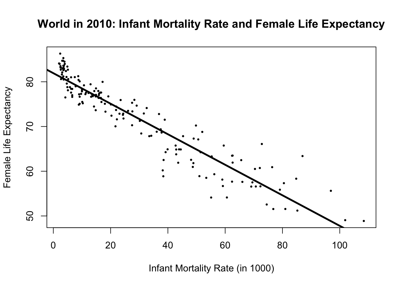
8.4 Visualising the Regression Line
We can visually display the estimated regression line on the scatter plot. We just need to use the abline() function. Let’s feed the reg_mod1 into the abline() function. I will also specify the thickness of the line by using the argument lwd. It will make the line three times thicker for better visibility.
# Plotting the regression line ####
plot(df$Infant_Mortality_Rate, df$Life_exp_female,
     main = "World in 2010: Infant Mortality Rate and Female Life Expectancy",
     xlab = "Infant Mortality Rate (in 1000)",
     ylab = "Female Life Expectancy",
     pch = 16, # change points from hollow circles to filled circle
     cex = 0.5 # make the points smaller (half in size)
     )
# add the regression line on to the plot:
abline(reg_mod1, # reg_mod1 is the main input: intercept and slope.
       lwd = 3   # lwd is for making the line thicker
) 
8.5 predict() Function
As we have seen, the regression equation allows us to calculate predicted values of \(Y\) (Life_exp_female, in this example) given \(X\) (Infant_Mortality_Rate). We could calculate predicted values one-by-one as we did for X values of 1, 2, and 10. However, asking R to do it for us is much faster and easier.
For this objective, we will use the predict() function, which returns the predicted (or expected) values of \(Y\) given the explanatory variable(s).
If you directly plug our model (reg_mod1) into the predict() function, the model will generate predicted values of the outcome variable for realizations of Infant_Mortality_Rate (i.e. actual data points). Let’s display it on our screen.
# Predicted values of Y given X ####
predict(reg_mod1)
These are predictions based on our regression model and actual measurements Infant_Mortality_Rate. We can also give hypothetical values of Infant_Mortality_Rate. Previously, we plugged in 1, 2, and 10. Let’s do the same by using predict().
# predict by giving new (hypothetical) data points ####
# this is our initial predictions for X values of 1, 2 and 10

# create a new data frame in which we are going to store our hypothetical Infant_Mortality_Rate values:
df_pred_ini <-  data.frame(Infant_Mortality_Rate = c(1, 2, 10))

# see this data frame: ini is abb for initial
df_pred_ini
Infant_Mortality_Rate
1 1
2 2
3 10# df_pred_initial is just a new data frame
# it holds hypothetical Infant_Mortality_Rate values
View(df_pred_ini)Next, plug in this new data to the predict() function.
# prediction using 'new' data:
predict(reg_mod1, newdata = df_pred_ini)
1 2 3
81.58465 81.24327 78.51224 # store it in the new df
df_pred_ini$predicted_fem_life_exp <- predict(reg_mod1, newdata = df_pred_ini)# new data frame now holds:
# predicted infant mortality rates given hypothetical Infant_Mortality_Rate
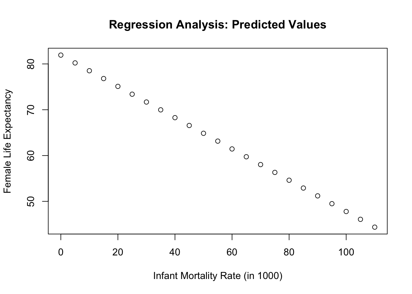
View(df_pred_ini)In this example, we just used a three hypothetical values for Infant_Mortality_Rate, namely 1,2, and 10. These are the values we used in our ‘manuel calculations’ using the regression equation and \(\alpha\) and \(\beta\) coefficients. We can plug in large number of hypothetical values if we like.
# A series of hypothetical values
x <- seq(from = 0, to = 110, by = 5)

# put it into a data frame
df_pred_big <- data.frame(Infant_Mortality_Rate = x)

# predictions
df_pred_big$pred_fem_life_exp <- predict(reg_mod1, newdata = df_pred_big)
See your predicted values.
# See the df_pred_big
View(df_pred_big)
Note that these predicted values are always on the regression line! If you plot them, they will form a line (i.e., the regression line).
plot(x = df_pred_big$Infant_Mortality_Rate,
     y = df_pred_big$pred_fem_life_exp,
     main = "Regression Analysis: Predicted Values",
     xlab = "Infant Mortality Rate (in 1000)",
     ylab = "Female Life Expectancy"
     )
8.6 Regression Prediction Error
Next, we will calculate the errors (also known as residuals), which are the differences between the actual data points (i.e., realizations) of \(Y\) and the predicted values of \(Y\).
\[ Error = Actual \; Y - Predicted \; Y \]
For simplification of notation, we use \(e\) for error, \(Y\) for actual data points and Y-hat (\(\hat{Y}\)) for predictions.
\[ e = y - \hat{y} \]
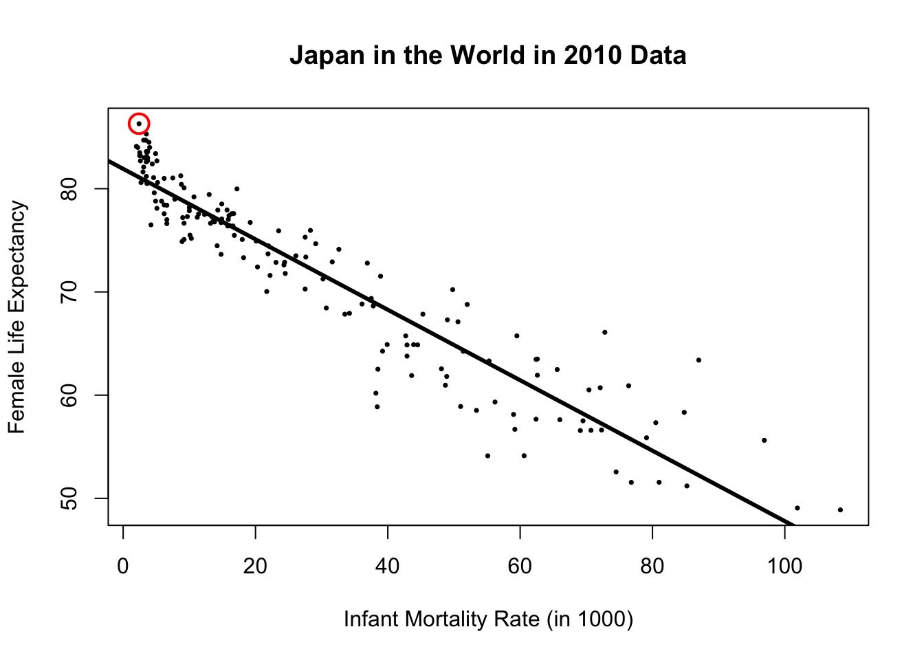
For example, let’s look at Japan. What is Japan’s Infant_Mortality_Rate and Fem_Life_Exp? We can quickly ask R to bring it for us.
# Infant Mortality Rate for Japan :
# bring me Mortality rate such that Country Name is Japan:
df$Infant_Mortality_Rate[df$Country_Name == "Japan"]
[1] 2.4# Female Life Expectancy for Japan
# bring me Female Life Expectancy such that Country Name is Japan:
df$Life_exp_female[df$Country_Name == "Japan"][1] 86.3Japan’s actual Female Life Expectancy is \(86.3\). We are going to compare this to the predicted value. Let’s calculate the predicted value for Japan:
\[\begin{align*} \hat{y} &= 81.93 - 0.34 * 2.4 \\ &= 81.11 \end{align*}\]
I am very bad with calculations, so let’s ask R if we did it correctly.
# x value for Japan:
x_jpn   <- df$Infant_Mortality_Rate[df$Country_Name == "Japan"]

# make it a data frame to feed into predict() function:
df_jpn  <- data.frame(Infant_Mortality_Rate = x_jpn)

# use the predict function:
predict(reg_mod1, newdata = df_jpn) |> round(2)
1
81.11 Now we can calculate the error! It is the actual minus the predicted:
\[\begin{align*} e &= y - \hat{y} \\ &= 86.3 - 81.11 \\ &= 5.19 \end{align*}\]
This difference is illustrated in Figure 8.3, where Japan’s data point is highlighted with a red circle. Notice that it is positioned above the corresponding regression line. Specifically, Japan’s actual \(Y\) value is \(5.19\) years higher than its predicted value.
Show/Hide R Code for Plot for Japan
# The code for generating Figure 8.3

# Usual scatter plot:
plot(df$Infant_Mortality_Rate, df$Life_exp_female,
     main = "Japan in the World in 2010 Data",
     xlab = "Infant Mortality Rate (in 1000)",
     ylab = "Female Life Expectancy",
     pch = 16,
     cex = 0.5
     )

# add the regression line on to the plot:
abline(reg_mod1, # reg_mod1 is the main input: intercept and slope.
       lwd = 3   # lwd is for making the line thicker
       )

# now highlight the data point for Japan:
points(x = df$Infant_Mortality_Rate[df$Country_Name == "Japan"], # x value for Japan
       y = df$Life_exp_female[df$Country_Name == "Japan"], # y value for Japan
       pch = 1, # default pch will circle the point
       lwd  = 2,  # make the circle thicker
       cex = 2,  # make the circle bigger
       col = "red" # make the circle red!
       )
8.6.1 Residual (error) for all countries
We used Japan as an illustrative example. Next, we will calculate the residuals (or errors) for all countries. We need to be careful because of handling any missing data. If you try to store the predicted values in your original data frame, your code will not run and you will get an error message.
df$yhat <- predict(reg_mod1)Error in `$<-.data.frame`(`*tmp*`, yhat, value = c(`1` = 59.5315545866218, : replacement has 165 rows, data has 166The error message says the replacement has 165 rows, data has 166. Let’s unpack this. Our original data frame has 166 observations (rows).
# number of observations:
nrow(df)
[1] 166However, the model returns 165 predicted values.
# the number of predicted values
predict(reg_mod1) |> length()
[1] 165Why is there a difference? Recall that one observation was missing for Infant_Mortality_Rate.
# summary of variables of interest
summary(df$Infant_Mortality_Rate)
Min. 1st Qu. Median Mean 3rd Qu. Max. NA's
2.00 7.50 19.20 29.25 48.10 108.40 1 When R is running the requested regression, it automatically handles missingness by skipping the rows where at least one measurement is missing. In this case, the row for Kosovo is skipped because its Infant_Mortality_Rate is not available.
While working with residuals, it is practical to create a smaller data frame with only the variables that are used in the regression. We can also remove the any missing observations.
# Using tidyverse select only the variables of interest (and country name to identify observations):
df_reg <- df |>
  select(Country_Name, Life_exp_female, Infant_Mortality_Rate) |>
  na.omit() # remove rows that contain any missingness

# check the number of rows:
# it should be one lower than the original data
# because one row (for Kosovo) is removed
nrow(df_reg)
[1] 165Let’s try again to generate predicted values.
# predicted values
df_reg$predicted <- predict(reg_mod1, newdata = df_reg)
# see your new data frame with predicted values:
View(df_reg)It is time to calculate the residuals for all countries.
# calculate the residuals (errors):
df_reg$error <- df_reg$Life_exp_female - df_reg$predicted
You can explore your model’s predictions by examining the errors. For instance, which countries does the model predict inaccurately? In other words, which countries have a Life_exp_fem that is higher (or lower) than expected, given their Infant_Mortality_Rate? We can explore these.
8.7 Task #1: Lecture Example (Marks and Study Time)
Using the data from the lecture slides, answer the questions below using R.
# lecture example data:
lect <- data.frame(
  mark = c(37, 30, 45, 48, 63, 57, 65, 55, 50, 70),
  study_time = c(rep(1, 4), rep(4, 6))
)- Perform a regression of
markonstudy_time. Report the alpha and beta. - I plan to study 7 hours in the next exam. Using the regression model, calculate my expected mark?
- What is my expected mark if I do not study at all?
- What is the mean of
mark?- unconditional mean
- mean conditional on 1 hour of
study_time - mean conditional on 4 hours of
study_time
- Plot
markandstudy_time. X-axis should span from 0 to 6 hours of study. Y-axis should be from 0 to 100. Draw the regression line. - Challenge: On the plot you created for question 5, show that conditional means are on the regression line.
Answers
- Perform a regression of
markonstudy_time. Report the alpha and beta.
Show the answer for Question 1
# regression for task 1
reg_t1 <- lm(mark ~ study_time, data = lect)
reg_t1
# The intercept is 33.33
# The beta is 6.67- I plan to study 7 hours in the next exam. Using the regression model, calculate my expected mark?
Show the answer for Question 2
predict(reg_t1, newdata = data.frame(study_time = 7))- What is my expected mark if I do not study at all?
Show the answer for Question 3
# This is the intercept. It is 33.333 but let's display it on screen:
reg_t1$coefficients[1]- What is the mean of
mark? Unconditional and conditional means.
Show the answer for Question 4
# unconditional mean:
mean(lect$mark)

# mean conditional on X = 1:
mean(lect$mark[lect$study_time == 1])

# mean conditional on X = 4:
mean(lect$mark[lect$study_time == 4])- Plot
markandstudy_time. Draw a regression line.
Show the answer for Question 5
# plot:
plot(x = lect$study_time,
     y = lect$mark,
     xlim = c(0, 6),
     ylim = c(0, 100),
     xlab = "Study Time",
     ylab = "Mark",
     main = "Data: Example from the Lecture",
     pch = 16)
# add the regression line:
abline(reg_t1, lwd = 2)- Challenge: On the plot you created for question 5, show that the conditional means are on the regression line.
Show the answer for Question 6
# points for conditional means:
# first point for x = 1:
p1 <- data.frame(x = 1,
                 y = mean(lect$mark[lect$study_time == 1])
                 )

# second point for x = 4:
p2 <- data.frame(x = 4,
                 y = mean(lect$mark[lect$study_time == 4])
                 )

### plotting part ###
# the original plot:
plot(x = lect$study_time,
     y = lect$mark,
     xlim = c(0, 6),
     ylim = c(0, 100),
     xlab = "Study Time",
     ylab = "Mark",
     main = "Data: Example from the Lecture",
     pch = 16)
# add the regression line:
abline(reg_t1, lwd = 2)

# add the points:
points(x = p1$x, y = p1$y, col = "red", pch = 15) # points for X = 1
points(x = p2$x, y = p2$y, col = "red", pch = 15) # points for X = 4
8.8 Task #2: Female Life Expectancy and Male Life Expectancy
Run a regression of Life_exp_female on Life_exp_male and perform the following analyses:
- Interpret the regression coefficients.
- Visualise the regression line: Create a scatter plot of the data and overlay the regression line to illustrate the relationship.
- Calculate the predicted values of
Life_exp_female. Use the regression model to predictLife_exp_femalefor all countries based on theirLife_exp_male. - Calculate the errors (residuals): Compute the difference between the actual and predicted values of
Life_exp_female. - Identify countries with higher-than-expected
Life_exp_female: which countries haveLife_exp_femalemore than five years abo the predicted values, given theirLife_exp_male?. - Identify countries with lower-than-expected
Life_exp_female: which countries haveLife_exp_femalevalues more than two years below the predicted values, given theirLife_exp_male?.
Show the answer for Task 2
# regression:
reg_t2 <- lm(Life_exp_female ~ Life_exp_male, data = df)

# regression coefficients:
reg_t2

# One year (unit) increase in Life_exp_male is associated with 1.084 years of increase in Life_exp_female
# No need to try interpreting the intercept substantively.
# Intercept is not meaningful in this case. No substantive interpretation.
# Technically, when the life expectancy of men is 0 years old, the female life expectancy is -0.771 (this is not really meaningful).


# plot:
plot(df$Life_exp_male, df$Life_exp_female,
     xlab = "Male Life Expectancy",
     ylab = "Female Life Expectancy",
     pch = 16
     )
# add the regression line:
abline(lm(reg_t2), lwd = 3)

# Use the regression model to predict `Life_exp_female` for all countries based on their `Life_exp_male`:
df$predicted_fem_life <- predict(reg_t2)

# errors:
df$errors <- df$Life_exp_female - df$predicted_fem_life

# Which countries have `Life_exp_female` more than five years abo the predicted values, given their `Life_exp_male`?.
df$Country_Name[df$errors > 5]

# Which countries have `Life_exp_female` values more than two years below the predicted values, given their `Life_exp_male`?.
df$Country_Name[df$errors < -2]
8.9 Task #3: Challenge: Imputation
Recall that Kosovo’s Infant_Mortality_Rate is missing in the World in 2010 dataset. Using a simple regression model with Life_exp_female as the only predictor, estimate the Kosovo’s Infant_Mortality_Rate.
Tip: Unhide to see the tip
Predicted variable is the outcome variable.
Your outcome variable should be Infant_Mortality_Rate and your independent variable is Life_exp_female.
Answer for Task 3
# regression: outcome variable is Infant_Mortality_Rate
reg_t3 <- lm(Infant_Mortality_Rate ~ Life_exp_female, data = df)

# Prediction for Kosovo:
# isolate Kosovo's data :
Kosovo <- df[df$Country_Name == "Kosovo", ]

# variables of interest:
Kosovo <- Kosovo |> select(Country_Name, Infant_Mortality_Rate, Life_exp_female)
# see that Infant Mortality Rate is missing for Kosovo
View(Kosovo)

# predicted value
Kosovo$predicted_inf_mor <- predict(reg_t3, newdata = Kosovo)
Kosovo$predicted_inf_mor