names_pm <- c("Keir Starmer",
              "Rishi Sunak",
              "Liz Truss",
              "Boris Johnson",
              "Theresa May",
              "David Cameron",
              "Gordon Brown",
"Tony Blair")2 Data in R
Last week we started with a gentle introduction to R. We created a basic dataset, with the names of UK Prime Ministers and their respective birthdays.
Let’s remember the steps. First, we created an object called pm_names. We did this by using the function c() which refers to combine.
The object pm_names holds the information we feed into: the names of the Prime Ministers. Let’s check the object.
names_pm[1] "Keir Starmer" "Rishi Sunak" "Liz Truss" "Boris Johnson"
[5] "Theresa May" "David Cameron" "Gordon Brown" "Tony Blair" This is basically the names of the last eight UK Prime Ministers. The number in square brackets refers to an item’s position. For example [1] in front of Keir Starmer tells me that the first item in the object names_pm is Keir Starmer. Similarly the fifth item in names_pm is Theresa May.
Let’s recall the square brackets notation [] which is used to get a specific item from an object.
# First item in names_pm is "Keir Starmer"
names_pm[1]
[1] "Keir Starmer"# Fifth item in names_pm is "Theresa May"
names_pm[5][1] "Theresa May"# First and fifth item in the names_pm
names_pm[c(1,5)][1] "Keir Starmer" "Theresa May" # Fourth item in the names_pm
names_pm[4][1] "Boris Johnson"
Vectors
A series of information following each other is may called a vector. The object names_pm is a vector because it contains a series of information in a sequence. More specifically, names_pm is a vector of names. We will revisit the term vector.
Last week, we also created another object called birth_years, storing the information of birth years of each Prime Minister in names_pm. Also recall that the order of year of birth is important. For example, first item in birth_years should be Keir Starmers’s year of birth, second item should be Rishi Sunak’s, and so on.
birth_years <- c(1962, # Keir Starmer
                 1980, # Rishi Sunak
                 1975, # Liz Truss
                 1964, # Boris Johnson
                 1956, # Theresa May
                 1966, # David Cameron
                 1951, # Gordon Brown
                 1953  # Tony Blair)
                 )
The object birth_years is a numerical vector. It contains numbers. Let’s check the object.
birth_years[1] 1962 1980 1975 1964 1956 1966 1951 19532.1 Class of an object
R understand the differences between textual and numerical information. We can check the class of an object using the class() function.
# birth_years contain numerical information
class(birth_years)
[1] "numeric"# names_pm contain textual information, which is called character in R
class(names_pm)[1] "character"2.2 Length of an object
We typed names of last eight Prime Ministers and their respective birth years. The number of items in names_pm and birth_years should be both eight. We can see the number of items in a vector by the length() function.
# Number of items in a vector can be seen by length()

# Length of names_pm:
length(names_pm)
[1] 8# Length of birth_years:
length(birth_years)[1] 82.3 is equal to operator
You can ask R whether two things are equal to each other or not. To do so, we are going to use the == operator, which means is equal to.
# is equal to operator: ==

# is the length of names_pm equal to birth_years
length(names_pm) == length(birth_years)
[1] TRUEThe number of items in both objects (names_pm and birth_years) is the same because both vectors contain eight pieces of information.
How about the class of the objects?
# is the class of names_pm equal to birth_years
class(names_pm) == class(birth_years)
[1] FALSEThe class of the objects is not the same because names_pm contains textual information whereas birth_years contains numerical information.
2.4 Creating a simple dataset
Last week we created a simple spreadsheet that looked like the data shown in
We can achieve this by doing a column bind which refers to vertically binding two vectors and can be done using the cbind() function.
my_data <- cbind(names_pm, birth_years)

# let's check the object we created
my_data
names_pm birth_years
[1,] "Keir Starmer" "1962"
[2,] "Rishi Sunak" "1980"
[3,] "Liz Truss" "1975"
[4,] "Boris Johnson" "1964"
[5,] "Theresa May" "1956"
[6,] "David Cameron" "1966"
[7,] "Gordon Brown" "1951"
[8,] "Tony Blair" "1953" The first column in my_data is names_pm and the second column is birth_years. We have now two dimensions: columns and rows.
Recall that to ask R to bring a specific item in a two-dimensional object, such as a spreadsheet, we can use the square-brackets [] notation but we need to specify both dimension.
Rows and Columns in a Spreadsheet
First dimension refers to rows and second dimension refers to columns.
Let’s get the third row in second column.
# Third row in second column
my_data[3,2]
birth_years
"1975" To sum up, we bound two vectors by column. Each column is a vector. We can call these column vectors. To get the first column, names_pm, we can use the square brackets notation.
# Bring the first column
my_data[,1]
[1] "Keir Starmer" "Rishi Sunak" "Liz Truss" "Boris Johnson"
[5] "Theresa May" "David Cameron" "Gordon Brown" "Tony Blair" # Bring the second column
my_data[,2][1] "1962" "1980" "1975" "1964" "1956" "1966" "1951" "1953"To get a specific column vector, we left the first dimension unspecificed. Recall that the first dimension designates the row, so leaving it unspecified means everything.
We could also use column names instead of column numbers.
# Bring the column birth_years
my_data[,"birth_years"]
[1] "1962" "1980" "1975" "1964" "1956" "1966" "1951" "1953"# Bring the column names_pm
my_data[,"names_pm"][1] "Keir Starmer" "Rishi Sunak" "Liz Truss" "Boris Johnson"
[5] "Theresa May" "David Cameron" "Gordon Brown" "Tony Blair" We can do the same for rows. To get a row vector, use the squared bracket notation.
# Bring the first row
my_data[1, ]
names_pm birth_years
"Keir Starmer" "1962" # Bring the third row
my_data[3,] names_pm birth_years
"Liz Truss" "1975" # Bring the fourth row
my_data[4,] names_pm birth_years
"Boris Johnson" "1964" R will give you an error message if you go out of bounds.
# Bring the third column
my_data[,3]
Error in my_data[, 3]: subscript out of bounds# Bring the 10th row
# Bring the second column, ninth row
my_data[9,2]Error in my_data[9, 2]: subscript out of bounds2.5 Data frame
It is customary to keep a spreadsheet-like looking data (i.e., two-dimensional) as something called a data frame in R. Let’s check the class of my_data.
# Class of my_data
class(my_data)
[1] "matrix" "array" It looks like the class of my_data is matrix and array. Matrix is a two-dimensional array.
We can turn my_data into a data frame.
# Turn my_data into data frame
my_data <- as.data.frame(my_data)
# this just overwrote my_data as a data frame

# Check its class
class(my_data)
[1] "data.frame"In this module, we will primarily work with data frames.
Recall that we can use the $ notation when working with data frames.
# bring names_pm
my_data$names_pm
[1] "Keir Starmer" "Rishi Sunak" "Liz Truss" "Boris Johnson"
[5] "Theresa May" "David Cameron" "Gordon Brown" "Tony Blair" # bring birth_years
my_data$birth_years[1] "1962" "1980" "1975" "1964" "1956" "1966" "1951" "1953"# bring the third item in birth_years
my_data$birth_years[3][1] "1975"We can check the number of columns and the number of rows of our data frame by using ncol() and nrow() functions.
# number of columns
ncol(my_data)
[1] 2# number of rows
nrow(my_data)[1] 8A data frame, such as my_data, has two dimensions: rows and columns. Note that my_data has eight rows and two columns. We can use the dim() function to get the length of each dimension.
dim(my_data)[1] 8 22.6 Variable, Row, Observation
Let’s check some more terminology that is frequently used in data analysis.
A column vector typically shows a variable. A row vector typically shows an observation. A particular item, which is a cell in a spreadsheet, is a value. This is visualised in Figure 2.1.
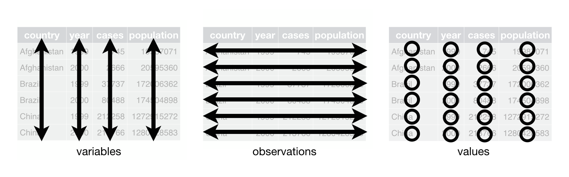
When data do not come in this format, we will carry out something called data wrangling and reorganize the data so that each column is a variable, each row is an observation and each cell is a value.
For simplicity, however, the datasets we are working on already come in this shape.
# A variable: a column (e.g., birth_years)
my_data$birth_years
[1] "1962" "1980" "1975" "1964" "1956" "1966" "1951" "1953"# An observation: a row (e.g., second row)
my_data[2,] names_pm birth_years
2 Rishi Sunak 1980# A particular value (e.g., third row of second column)
my_data[3,2][1] "1975"2.7 Numerical value stored as character
Let’s say we would like to calculate each person’s current age. We could simply tell R to subtract each birth year from current year (2024).
2024 - my_data$birth_yearsError in 2024 - my_data$birth_years: non-numeric argument to binary operatorInstead of the calculation, I get an error message: non-numeric argument to…! Let’s see what is going on.
# Check the variable of interest
my_data$birth_years
[1] "1962" "1980" "1975" "1964" "1956" "1966" "1951" "1953"birth_years is a vector of numbers but if you look closely, you will see that each number is shown within a pair of quotation mark. This is because R is keeping each number as text at the moment. Let’s look at the class of the object.
# Class of birth_years
class(my_data$birth_years)
[1] "character"Character means text. We are going to use as.numeric() function to tell R that information stored in birth_years is numerical, not text.
# Convert the variable to numerical
as.numeric(my_data$birth_years)
[1] 1962 1980 1975 1964 1956 1966 1951 1953Now quotation marks disappeared. Beware: I have not overwritten the variable yet. It is just displayed on my screen for one time only. I need to overwrite the existing version to make it a permanent change.
my_data$birth_years <- as.numeric(my_data$birth_years)This command tells R to:
- go and get the variable
birth_yearsinside the data framemy_data - convert it numeric
- take the numerical output and assign it over the variable
birth_yearsin the data framemy_data
Now birth_years should be numerical.
class(my_data$birth_years)[1] "numeric"Now, we can create the current age variable.
# Calculate the current age
2023 - my_data$birth_years
[1] 61 43 48 59 67 57 72 70# It is working. Let's assign this output to a new variable
my_data$age_current <- 2023 - my_data$birth_years
# Check my_data
my_data names_pm birth_years age_current
1 Keir Starmer 1962 61
2 Rishi Sunak 1980 43
3 Liz Truss 1975 48
4 Boris Johnson 1964 59
5 Theresa May 1956 67
6 David Cameron 1966 57
7 Gordon Brown 1951 72
8 Tony Blair 1953 702.8 Categorical data
I would like to add a variable showing the party of each Prime Minister. I can create a vector and add this as a column in my_data.
For example, Rishi Sunak is from Conservative Party, Liz Truss is also Conservative. Kier Starmer, Gordon Brown and Tony Blair are Labour.
We need a vector where the first item is Labour, followed by five Conservative, and two Labour at the end.
We could write it one by one in order. It would be long and cumbersome, but it would do the job.
parties_long_version <-  c("Labour", # first item Labour
                                "Conservative", # followed by five Conservative (1)
                                "Conservative", # (2)
                                "Conservative", # (3)
                                "Conservative", # (4)
                                "Conservative", # (5)
                                "Labour", # This corresponds to Gordon Brown
                                "Labour" # Finally, Tony Blair
                                )
Let’s check the object we created.
parties_long_version[1] "Labour" "Conservative" "Conservative" "Conservative" "Conservative"
[6] "Conservative" "Labour" "Labour" This looks good. I could assign it into a new column in my_data. But we are learning, so let’s try another and faster-to-write way.
Instead of repeating Conservative five times, I could use the repeat function: rep().
# rep() repeats an input n times
rep("Conservative", 5)
[1] "Conservative" "Conservative" "Conservative" "Conservative" "Conservative"Using this approach, I can build the vector again. I need one “Labour”, five “Conservative”, and two “Labour”, in this order. I need to combine them using (c).
parties_short_version <-  c("Labour",
                            rep("Conservative", 5),
                            rep("Labour", 2))
Let’s check the object we created
parties_short_version[1] "Labour" "Conservative" "Conservative" "Conservative" "Conservative"
[6] "Conservative" "Labour" "Labour" Both versions should be the same, meaning parties_long_version should be equal to parties_short_version.
parties_long_version == parties_short_version [1] TRUE TRUE TRUE TRUE TRUE TRUE TRUE TRUENow, let’s put it into my data frame.
my_data$party <- parties_short_versionLet’s check the data frame.
my_data names_pm birth_years age_current party
1 Keir Starmer 1962 61 Labour
2 Rishi Sunak 1980 43 Conservative
3 Liz Truss 1975 48 Conservative
4 Boris Johnson 1964 59 Conservative
5 Theresa May 1956 67 Conservative
6 David Cameron 1966 57 Conservative
7 Gordon Brown 1951 72 Labour
8 Tony Blair 1953 70 Labour2.9 Counting frequencies using table ()
Let’s see how many individuals from each party is in my data frame. You could count it one by one in a small data set such as this one. I can see that there are 5 Conservatives and three Labour, but imagine that it was a large dataset where counting manually was not an option.
We can use table() function to achieve this.
table(my_data$party)
Conservative       Labour
           5            3
2.10 Saving data
In the final step, we will learn how to save a data frame such as my_data for future use. We have a few options:
- Write my_data into a spreadsheet-like file.
- Save the whole R environment with all the objects inside.
We will cover option #1 here.
You have probably used Microsoft Excel (or Google Sheets) to work on spreadsheets before. There are different spreadsheet file types (such as Excels .xlsx), but the most common and compatible one is .csv, which stands for comma separated values. This is basically plain text that any computer and most electronic devices can open.
write.csv(x = my_data, file = "my_first_file.csv", row.names = F)This should create a file somewhere in your computer, more precisely, in your working directory. Let’s see where it has saved the file by looking at the working directory.
getwd()2.11 Working directory
getwd() means get working directory. Working directory is your default file path. This is where R looks for files and saves any output.
Working directory can be different in each computer. R Studio has nice tools for navigation.
You can directly go to your working directory through Files tab (usually in right bottom corner) and using the More drop-down menu. Under there there are a few options:
- Set as working directory: sets your working directory as the current directory shown in Files
- Go to working directory: takes you to current working directory
If you click on go to working directory, you should see my_first_file.csv here.
It is a good idea to create a new directory (folder for Windows) for this module. Your folder names should be simple and easy to write. For example: research_methods is a good name.
Try not to use space in file names. Underscore or dash are better alternatives. Also, I encourage always using lowercase for file names, which also goes for object names in R.
You can use your operating system to create this directory. You could also use R Studio’s Files tab. Put this folder somewhere easy to access.
Let’s save your R script. You can use drop-down menu: File >> Save OR simply by using the keyboard shortcut .
Give an intuitive name to your script. For example, learn_02.R is a good name.
It is generally good idea to keep your data in a sub-directory named data. Create such a directory and move my_first_file.csv there.
Next week, we will continue with a simple dataset, which will be available on Blackboard.